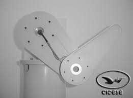
trajectory-simulation-pelican-robot

Trajectory simulation of the Pelican Prototype Robot of the CICESE Research Center, Mexico. The position control used was PD control with gravity compensation and the 4th order Runge-Kutta method.

Project maintained by JCLArriaga5 Hosted on GitHub Pages — Theme by mattgraham

Pelican Experimental Robot Trajectory Simulation

License size

Trajectory simulation of the Pelican Prototype Robot of the CICESE Research Center, Mexico. The position control used was PD control with gravity compensation and the 4th order Runge-Kutta method.

Use the repository

$ git clone https://github.com/JCLArriaga5/trajectory-simulation-pelican-robot.git

Enter the path where the repository was cloned and install the dependencies with the following command:

$ pip install -r requirements.txt

Simulation

You can review the simulation carried out in a Colab notebook using the functions created in probot, by clicking here:

or use the shell/command prompt for run simulation in probot Python File:

:~/trajectory-simulation-pelican-robot$ cd pelcnrbt/
:~/trajectory-simulation-pelican-robot/pelcnrbt$ python probot.py

The simulation must be in order:

# Desired position
pd = [0.26, 0.13]
# Gains
kp = [[30.0, 0.0],
      [0.0, 30.0]]
kv = [[7.0, 0.0],
      [0.0, 3.0]]
# Initial values of angles and velocities
qi = [0.0, 0.0]
vi = [0.0, 0.0]
ti = 0.0
tf = 1.0

sim = pelican_robot(pd, kp, kv, control_law='PD-GC')
qsf, qpsf = sim.run(ti, qi, vi, tf)

Kp, Kv are symmetric positive definite and selected by the designer and are commonly referred to as position gain and velocity (or derivative) gain, respectively. In form:

Kp = diag{kp} = diag{30, 30} [Nm/rad]
Kv = diag{kv} = diag{7, 3} [Nm/rad]

the qi angles were set to zero to start from home position in this case, if you want it to start from another position you can use the inverse_k function in utils.py which is the robot inverse kinematics which returns the values of q1 and q2 for the position you want:

from utils import inverse_k

qi = inverse_k(px, py)
# px is the desired x-coordinate
# py is the desired y-coordinate

Once the simulation values have been generated by run you can use the functions to graph the results.

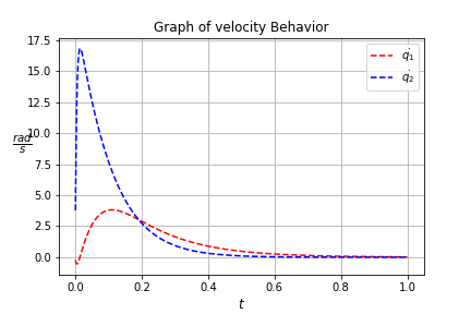
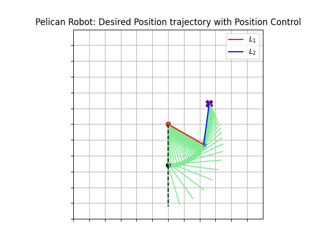
Images for desired position (0.26, 0.13)

Graph of error: The graph shows how the error of the angles for the desired position was reduced by the controller. The errors shown in the graph are a product of the friction phenomenon that has not been included in the dynamics of the robot.

sim.plot_q_error()

Graph of velocities behavior: The graph shows how the speed of each link behaved until reaching the desired position

sim.plot_velocity_bhvr()

Graph of desired position trajectory

sim.plot_trajectory(50)

Simulation Animated

If you want to see the animation of the trajectory to the desired position and the behavior of the error during the set time, use the parameter display=True in the RK4 function, as shown:

Note: Once the simulation values have been generated, inside sim.run code when the number of total iterations done, there will get values and show animation.

Note: Animation is not showing in Google Colab

sim = pelican_robot(pd, kp, kv, control_law='PD-GC')
qsf, qpsf = sim.run(ti, qi, vi, tf, display=True)

References

Kelly, R., Davila, V. S., & Perez, J. A. L. (2006). Control of robot manipulators in joint space. Springer Science & Business Media.

“Case Study: The Pelican Prototype Robot.” Control of Robot Manipulators in Joint Space, Springer-Verlag, 2005, pp. 113–32. DOI.org (Crossref), https://doi.org/10.1007/1-85233-999-3_6.